Feature Extraction
The first stage in consists in transforming the raw data into a uniform data matrix which will subsequently be given as input to the learning algorithm.
resspect can handle FITS format data from the RESSPECT project, csv data from the Photometric LSST Astronomical Classification Challenge (PLAsTiCC) and text-like data from the SuperNova Photometric Classification Challenge (SNPCC).
Before starting any analysis, you need to choose a feature extraction method, all light curves will then be handdled by this method. In the examples below we used the Bazin feature extraction method (Bazin et al., 2009 ) or the Malanchev feature extraction method (Malanchev et al., 2021 ).
Load 1 light curve:
For SNPCC using Bazin features:
The raw data looks like this:
SURVEY: DES
SNID:   729076
IAUC:    UNKNOWN
PHOTOMETRY_VERSION: DES
SNTYPE:  -9
FILTERS: griz
RA:      0.500000  deg
DECL:    -43.000000  deg
MAGTYPE: LOG10
MAGREF:  AB
FAKE:    2   (=> simulated LC with snlc_sim.exe)
MWEBV:   0.0111    MW E(B-V)
REDSHIFT_HELIO:   0.21624 +- 0.03840  (Helio, z_best)
REDSHIFT_FINAL:   0.21624 +- 0.03840  (CMB)
REDSHIFT_SPEC:    -9.00000 +- 9.00000
REDSHIFT_STATUS: OK

HOST_GALAXY_GALID:   18506
HOST_GALAXY_PHOTO-Z:   0.2162  +- 0.0384


SIM_MODEL:  NONIA  10  (name index)
SIM_NON1a:      27   (non1a index)
SIM_COMMENT:  SN Type = II , MODEL = SDSS-015339
SIM_LIBID:  4
SIM_REDSHIFT:  0.1838
SIM_HOSTLIB_TRUEZ:  0.1800  (actual Z of hostlib)
SIM_HOSTLIB_GALID:  18506
SIM_DLMU:      39.752602  mag   [ -5*log10(10pc/dL) ]
SIM_RA:        0.500000 deg
SIM_DECL:      -43.000000 deg
SIM_MWEBV:   0.0084   (MilkyWay E(B-V))
SIM_PEAKMAG:   21.05  21.21  21.24  21.67  (griz obs)
SIM_EXPOSURE:     1.0    1.0    1.0    1.0  (griz obs)
SIM_PEAKMJD:   56239.878906  days
SIM_SALT2x0:   1.256e-16
SIM_MAGDIM:    0.000
SIM_SEARCHEFF_MASK:  3  (bits 1,2=> found by software,humans)
SIM_SEARCHEFF:  1.0000  (spectro-search efficiency (ignores pipelines))
SIM_TRESTMIN:   -38.74   days
SIM_TRESTMAX:    66.02   days
SIM_RISETIME_SHIFT:   0.0 days
SIM_FALLTIME_SHIFT:   0.0 days

SEARCH_PEAKMJD:   56240.938


# ============================================
# TERSE LIGHT CURVE OUTPUT:
#
NOBS: 77
NVAR: 9
VARLIST:  MJD  FLT FIELD   FLUXCAL   FLUXCALERR   SNR    MAG     MAGERR  SIM_MAG
OBS:  56194.012  g NULL   1.309e+01   6.204e+00   2.11   99.000    5.000   98.974
OBS:  56194.016  r NULL  -4.680e+00   3.585e+00  -1.31   99.000    5.000   99.014
OBS:  56194.023  i NULL  -1.936e+00   6.147e+00  -0.31   99.000    5.000   98.972
OBS:  56194.031  z NULL   2.477e+01   1.509e+01   1.64   99.000    5.000   99.050
OBS:  56198.992  g NULL   9.439e+00   1.868e+01   0.51   99.000    5.000   98.974
OBS:  56199.000  r NULL  -8.159e+00   9.049e+00  -0.90   99.000    5.000   99.014
OBS:  56199.008  i NULL  -1.962e+00   1.181e+01  -0.17   99.000    5.000   98.972
You can load this data using:
1>>> from resspect import BazinFeatureExtractor
2
3>>> path_to_lc = 'data/SIMGEN_PUBLIC_DES/DES_SN729076.DAT'
4
5>>> lc = BazinFeatureExtractor()             # create light curve instance
6>>> lc.load_snpcc_lc(path_to_lc)             # read data
This allows you to visually inspect the content of the light curve:
1>>> lc.photometry                            # check structure of photometry
2          mjd band     flux  fluxerr   SNR
3 0   56194.012       g       13.090  6.204   2.11    99.000  5.000
4 1   56194.016       r       -4.680  3.585   -1.31   99.000  5.000
5 ... ...     ...     ...     ...     ...     ...     ...
6 75  56317.051       i       173.200 7.661   22.60   21.904  0.049
7 76  56318.035       z       141.000 13.720  10.28   22.127  0.111
For SNPCC using Malanchev features:
You can load the data using:
1>>> from resspect import MalanchevFeatureExtractor
2
3>>> path_to_lc = 'data/SIMGEN_PUBLIC_DES/DES_SN729076.DAT'
4
5>>> lc = MalanchevFeatureExtractor()         # create light curve instance
6>>> lc.load_snpcc_lc(path_to_lc)             # read data
This allows you to visually inspect the content of the light curve:
1>>> lc.photometry                            # check structure of photometry
2          mjd band     flux  fluxerr   SNR
3 0   56194.012       g       13.090  6.204   2.11    99.000  5.000
4 1   56194.016       r       -4.680  3.585   -1.31   99.000  5.000
5 ... ...     ...     ...     ...     ...     ...     ...
6 75  56317.051       i       173.200 7.661   22.60   21.904  0.049
7 76  56318.035       z       141.000 13.720  10.28   22.127  0.111
Fit 1 light curve:
For SNPCC using Bazin features:
In order to feature extraction in one specific filter, you can do:
1>>> lc.fit('r')
2[514.92432962  -5.99556655  40.59581991  40.03343317   3.74307339]
The designation for each parameter are stored in:
1>>> lc.features_names
2['a', 'b', 't0', 'tfall', 'trise']
It is possible to perform the fit in all filters at once and visualize the result using:
1>>> lc.fit_all()                            # perform fit in all filters
2>>> lc.plot_fit(save=True, show=True,
3>>>             output_file='plots/SN' + str(lc.id) + '_flux.png')   # save to file
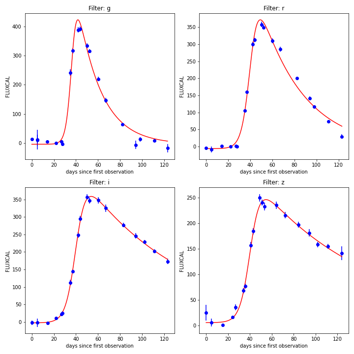
Example of light curve from SNPCC simulations.
This can be done in flux as well as in magnitude:
1>>> lc.plot_fit(save=False, show=True, unit='mag')
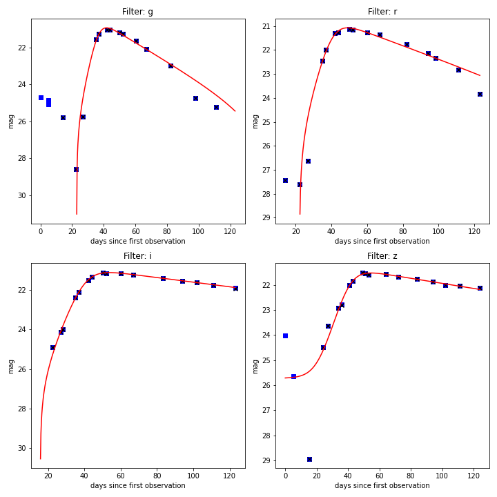
Example of light from SNPCC data.
Ocasionally, it is necessary to extrapolate the fitted light curve to a latter epoch – for example, in case we want to estimate its magnitude at the time of spectroscopic measurement (details in the time domain preparation section ).
Before deploying large batches for pre-processing, you might want to visualize how the extrapolation behaves for a few light curves. This can be done using:
1>>> # define max MJD for this light curve
2>>> max_mjd = max(lc.photometry['mjd']) - min(lc.photometry['mjd'])
3
4>>> lc.plot_fit(save=False, show=True, extrapolate=True,
5>>>                   time_flux_pred=[max_mjd+3, max_mjd+5, max_mjd+10])
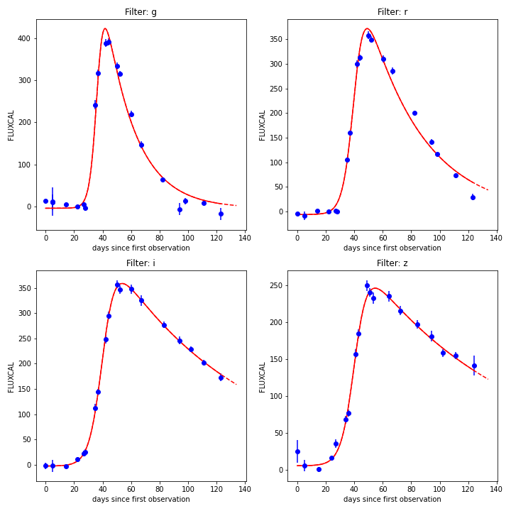
Example of extrapolated light from SNPCC data.
For SNPCC using Malanchev features:
In order to feature extraction in one specific filter, you can do:
1>>> lc.fit('r')
2[1.03403418e+00, 3.60823443e+02, 7.24896424e+02, 8.86255944e-01,
3 6.03107809e+01, 1.23027000e+02, 2.50709726e+02, 6.38344483e+01,
4 5.19719109e+01, 6.31578947e-01, 1.22756021e+00, 2.41334828e-02,
5 6.15343688e+02]
The designation for each parameter are stored in:
1>>> lc.features_names
2['anderson_darling_normal', 'inter_percentile_range_5', 'chi2',
3 'stetson_K', 'weighted_mean', 'duration', 'otsu_mean_diff',
4 'otsu_std_lower', 'otsu_std_upper', 'otsu_lower_to_all_ratio',
5 'linear_fit_slope', 'linear_fit_slope_sigma', 'linear_fit_reduced_chi2']
It is possible to perform the fit in all filters at once:
1>>> lc.fit_all() # perform fit in all filters
For PLAsTiCC:
Reading only 1 light curve from PLAsTiCC requires an object identifier. This can be done by:
 1>>> import pandas as pd
 2
 3>>> path_to_metadata = '~/plasticc_train_metadata.csv'
 4>>> path_to_lightcurves = '~/plasticc_train_lightcurves.csv.gz'
 5
 6# read metadata for the entire sample
 7>>> metadata = pd.read_csv(path_to_metadata)
 8
 9# check keys
10>>> metadata.keys()
11Index(['object_id', 'ra', 'decl', 'ddf_bool', 'hostgal_specz',
12       'hostgal_photoz', 'hostgal_photoz_err', 'distmod', 'mwebv', 'target',
13       'true_target', 'true_submodel', 'true_z', 'true_distmod',
14       'true_lensdmu', 'true_vpec', 'true_rv', 'true_av', 'true_peakmjd',
15       'libid_cadence', 'tflux_u', 'tflux_g', 'tflux_r', 'tflux_i', 'tflux_z',
16       'tflux_y'],
17     dtype='object')
18
19# choose 1 object
20>>> snid = metadata['object_id'].values[0]
21
22# create light curve object and load data
23>>> lc = BazinFeatureExtractor()
24>>> lc.load_plasticc_lc(photo_file=path_to_lightcurves, snid=snid)
Processing all light curves in the data set
There are 2 way to perform the Bazin fits for all three data sets. Using a python interpreter,
For SNPCC using Bazin features:
1>>> from resspect import fit_snpcc
2
3>>> path_to_data_dir = 'data/SIMGEN_PUBLIC_DES/'            # raw data directory
4>>> features_file = 'results/Bazin.csv'                     # output file
5>>> feature_extractor = 'bazin'
6
7>>> fit_snpcc(path_to_data_dir=path_to_data_dir, features_file=features_file, feature_extractor=feature_extractor)
For SNPCC using Malanchev features:
1>>> from resspect import fit_snpcc
2
3>>> path_to_data_dir = 'data/SIMGEN_PUBLIC_DES/'            # raw data directory
4>>> features_file = 'results/Malanchev.csv'                 # output file
5>>> feature_extractor = 'malanchev'
6
7>>> fit_snpcc(path_to_data_dir=path_to_data_dir, features_file=features_file, feature_extractor=feature_extractor)
For PLAsTiCC:
 1>>> from resspect import fit_plasticc
 2
 3>>> path_photo_file = '~/plasticc_train_lightcurves.csv'
 4>>> path_header_file = '~/plasticc_train_metadata.csv.gz'
 5>>> output_file = 'results/PLAsTiCC_Bazin_train.dat'
 6>>> feature_extractor = 'bazin'
 7
 8>>> sample = 'train'
 9
10>>> fit_plasticc(path_photo_file=path_photo_file,
11>>>              path_header_file=path_header_file,
12>>>              output_file=output_file,
13>>>              feature_extractor=feature_extractor,
14>>>              sample=sample)
The same result can be achieved using the command line:
1# for SNPCC
2>>> fit_dataset -s SNPCC -dd <path_to_data_dir> -o <output_file>
3
4# for PLAsTiCC
5>>> fit_dataset -s <dataset_name> -p <path_to_photo_file>
6         -hd <path_to_header_file> -sp <sample> -o <output_file>