Active Learning loop
Details on running 1 loop
Once the data has been pre-processed, analysis steps 2-4 can be performed directly using the DataBase object.
For start, we can load the feature information:
1>>> from resspect import DataBase
2
3>>> path_to_features_file = 'results/Bazin.csv'
4
5>>> data = DataBase()
6>>> data.load_features(path_to_features_file, feature_extractor='bazin', screen=True)
7Loaded  21284  samples!
Notice that this data has some pre-determine separation between training and test sample:
1>>> data.metadata['orig_sample'].unique()
2array(['test', 'train'], dtype=object)
You can choose to start your first iteration of the active learning loop from the original training sample flagged int he file OR from scratch. As this is our first example, let’s do the simple thing and start from the original training sample. The code below build the respective samples and performs the classification:
 1>>> data.build_samples(initial_training='original', nclass=2, screen=True)
 2** Inside build_orig_samples: **
 3   Training set size:  1093
 4   Test set size:  20191
 5   Validation set size:  20191
 6   Pool set size:  20191
 7      From which queryable:  20191
 8
 9>>> data.classify(method='RandomForest')
10>>> data.classprob                        # check classification probabilities
11array([[0.461, 0.539],
12       [0.346, 0.654],
13       ...,
14       [0.398, 0.602],
15       [0.396, 0.604]])
Hint
If you wish to start from scratch, just set the initial_training=N where N is the number of objects in you want in the initial training. The code will then randomly select N objects from the entire sample as the initial training sample. It will also impose that at least half of them are SNe Ias.
For a binary classification, the output from the classifier for each object (line) is presented as a pair of floats, the first column corresponding to the probability of the given object being a Ia and the second column its complement.
Given the output from the classifier we can calculate the metric(s) of choice:
1>>> data.evaluate_classification(metric_label='snpcc')
2>>> print(data.metrics_list_names)           # check metric header
3['acc', 'eff', 'pur', 'fom']
4
5>>> print(data.metrics_list_values)          # check metric values
6[0.5975434599574068, 0.9024767801857585,
70.34684684684684686, 0.13572404702012383]
Running a number of iterations in sequence
We provide a function where all the above steps can be done in sequence for a number of iterations.
In interactive mode, you must define the required variables and use the resspect.learn_loop function:
 1>>> from resspect.learn_loop import  learn_loop
 2
 3>>> nloops = 1000                                  # number of iterations
 4>>> method = 'bazin'                               # only option in v1.0
 5>>> ml = 'RandomForest'                            # classifier
 6>>> strategy = 'RandomSampling'                    # learning strategy
 7>>> input_file = 'results/Bazin.csv'               # input features file
 8>>> metric = 'results/metrics.csv'                 # output metrics file
 9>>> queried = 'results/queried.csv'                # output query file
10>>> train = 'original'                             # initial training
11>>> batch = 1                                      # size of batch
12
13>>> learn_loop(nloops=nloops, features_method=method, classifier=ml,
14>>>            strategy=strategy, path_to_features=input_file, output_metrics_file=metric,
15>>>            output_queried_file=queried, training=train, batch=batch)
Alternatively you can also run everything from the command line:
>>> run_loop -i <input features file> -b <batch size> -n <number of loops>
>>>             -m <output metrics file> -q <output queried sample file>
>>>             -s <learning strategy> -t <choice of initial training>
Active Learning loop in time domain
Considering that you have previously prepared the time domain data, you can run the active learning loop
following the same algorithm described in Ishida et al., 2019 by using the resspect.time_domain_loop module.
Note
The code below requires a file with features extracted from full light curves from which the initial sample will be drawn.
 1>>> from resspect import time_domain_loop
 2
 3>>> days = [20, 180]                                # first and last day of the survey
 4>>> training = 'original'                           # if int take int number of objs
 5                                                    # for initial training, 50% being Ia
 6
 7>>> strategy = 'UncSampling'                        # learning strategy
 8>>> batch = 1                                       # if int, ignore cost per observation,
 9                                                    # if None find optimal batch size
10
11>>> sep_files = False                               # if True, expects train, test and
12                                                    # validation samples in separate filess
13
14>>> path_to_features_dir = 'results/time_domain/'   # folder where the files for each day are stored
15
16>>> # output results for metrics
17>>> output_metrics_file = 'results/metrics_' + strategy + '_' + str(training) + \
18                       '_batch' + str(batch) +  '.csv'
19
20>>> # output query sample
21>>> output_query_file = 'results/queried_' + strategy + '_' + str(training) + \
22                        '_batch' + str(batch) +  '.csv'
23
24>>> path_to_ini_files = {}
25
26>>> # features from full light curves for initial training sample
27>>> path_to_ini_files['train'] = 'results/Bazin.csv'
28>>> survey='DES'
29
30>>> classifier = 'RandomForest'
31>>> n_estimators = 1000                             # number of trees in the forest
32
33>>> feature_extraction_method = 'bazin'
34>>> screen = False                                  # if True will print many things for debuging
35>>> fname_pattern = ['day_', '.csv']                # pattern on filename where different days
36                                                    # are stored
37
38>>> queryable= True                                 # if True, check brightness before considering
39                                                    # an object queryable
40
41>>> budgets = (6. * 3600, 6. * 3600)        # budget of 6 hours per night of observation
42
43
44>>> # run time domain loop
45>>> time_domain_loop(days=days, output_metrics_file=output_metrics_file,
46>>>                  output_queried_file=output_query_file,
47>>>                  path_to_ini_files=path_to_ini_files,
48>>>                  path_to_features_dir=path_to_features_dir,
49>>>                  strategy=strategy, fname_pattern=fname_pattern, batch=batch,
50>>>                  classifier=classifier,
51>>>                  sep_files=sep_files, budgets=budgets,
52>>>                  screen=screen, initial_training=training,
53>>>                  survey=survey, queryable=queryable, n_estimators=n_estimators,
54>>>                  feature_extraction_method=feature_extraction_method)
Make sure you check the full documentation of the module to understand which variables are required depending on the case you wish to run.
More details can be found in the corresponding docstring.
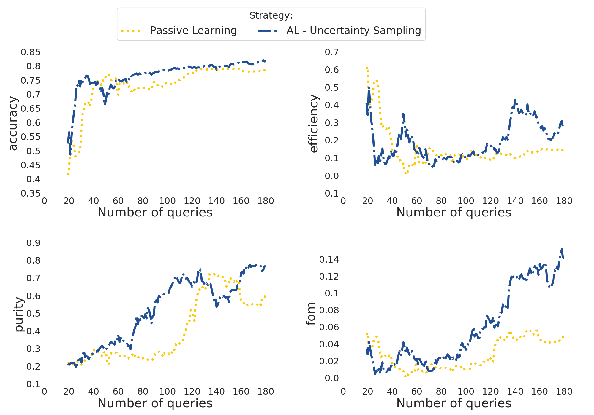
Once you ran one or more options, you can use the resspect.plot_results module, as described in the produce plots page.
The result will be something like the plot below (accounting for variations due to initial training).
Warning
At this point there is no Canonical sample option implemented for the time domain module.
Separate samples and Telescope resources
In a realistic situation, you might like to consider a more complex experiment design. For example, using a fixed validation sample and taking into account the time evolution of the transient and available resources for spectroscopic follow-up.
The RESSPECT reported an extensive study which takes into account many of the caveats related to realistic astronomical observations. The full report can be found at Kennamer et al., 2020.
In following the procedure described in Kennamer et al., 2020, the first step is to separate objects into train, test, validation and query samples.
 1>>> from resspect import sep_samples
 2>>> from resspect import read_features_fullLC_samples
 3
 4>>> # user input
 5>>> path_to_features = 'results/Bazin.csv'
 6>>> output_dir = 'results/'         # output directory where files will be saved
 7>>> n_test_val = 1000               # number of objects in each sample: test and validation
 8>>> n_train = 1500                  # number of objects to be separated for training
 9>>>                                 # this should be big enough to allow tests according
10>>>                                 # to multiple initial conditions
11
12>>> # read data and separate samples
13>>> all_data = pd.read_csv(path_to_features, index_col=False)
14>>> samples = sep_samples(all_data['id'].values, n_test_val=n_test_val,
15>>>                       n_train=n_train)
16
17>>> # read features and save them to separate files
18>>> for sample in samples.keys():
19>>>     output_fname = output_dir + sample + '_bazin.csv'
20>>>     read_features_fullLC_samples(samples[sample], output_fname,
21                                     path_to_features)
This will save samples to individual files. From these, only the query sample needs to be prepared for time domain, following instructions in Prepare data for Time Domain. Once that is done, there is only a few inputs that needs to be changed in the last call of the time_domain_loop function.
 1>>> sep_files = True
 2>>> batch = None                            # use telescope time budgets instead of
 3                                            # fixed number of queries per loop
 4
 5>>> budgets = (6. * 3600, 6. * 3600)        # budget of 6 hours per night of observation
 6
 7>>> path_to_features_dir = 'results/time_domain/'  # this is the path to the directory
 8                                                   # where the pool sample
 9                                                   # processed for time domain is stored
10
11>>> path_to_ini_files = {}
12>>> path_to_ini_files['train'] = 'results/train_bazin.csv'
13>>> path_to_ini_files['test'] = 'results/test_bazin.csv'
14>>> path_to_ini_files['validation'] = 'results/val_bazin.csv'
15
16
17>>> # run time domain loop
18>>> time_domain_loop(days=days, output_metrics_file=output_diag_file,
19>>>                  output_queried_file=output_query_file,
20>>>                  path_to_ini_files=path_to_ini_files,
21>>>                  path_to_features_dir=path_to_features_dir,
22>>>                  strategy=strategy, fname_pattern=fname_pattern,
23>>>                  batch=batch, classifier=classifier,
24>>>                  sep_files=sep_files, budgets=budgets,
25>>>                  screen=screen, initial_training=training,
26>>>                  survey=survey, queryable=queryable, n_estimators=n_estimators)
The same result can be achieved using the command line using the run_time_domain script:
1>>> run_time_domain -d <first day of survey> <last day of survey>
2>>>        -m <output metrics file> -q <output queried file> -f <features pool sample directory>
3>>>        -s <learning strategy> -t <training choice>
4>>>        -fl <path to initial training > -pv <path to validation> -pt <path to test>
Warning
Make sure you check the values of the optional variables as well!